Getting started
This notebook is meant to give a quick introduction into the main features and workflows of pyaerocom.
This includes brief introductions into the following features:
Finding model and observation data on the AeroCom servers (method
browse_database).Reading of gridded model data (
ReadGriddedclass).Reading of ungridded observation data (
ReadUngriddedclass).Working with gridded data (
GriddedDataclass).Working with ungridded data (
UngriddedDataclass).Retrieving and working with data from individual stations (
StationDataclass).Colocation of model data with all stations from an observation network.
It ends with a colocation of CAM53-Oslo model AODs both all-sky and clear-sky with Aeronet Sun V3 level 2 data.
Prerequisites
In order to run this notebook, you need to be connected to the AeroCom post processing servers (PPI).
If you have PPI (/lustre/) mounted on your local machine you need to update the basic data directory after importing pyaerocom as follows:
import pyaerocom as pya pya.const.BASEDIR = <path_where_lustre_is_mounted>
[1]:
import pyaerocom as pya
Initating pyaerocom configuration
Checking database access...
Checking access to: /lustre/storeA
Access to lustre database: True
Init data paths for lustre
Expired time: 0.021 s
Check data directory
By default, pyaerocom assumes that the AEROCOM database can be accessed (cf. top of flowchart), that is, it initiates all data query paths relative to the database server path names.
[2]:
pya.const.BASEDIR
[2]:
'/lustre/storeA/project/aerocom'
NOTE: Execution of the following lines will only work if you are connected to the AEROCOM data server or if you have access to the pyaerocom testdataset. The latter can be retrieved upon request (please contact jonasg@met.no).
Reading of and working with gridded model data (ReadGridded and GriddedData classes)
This section illustrates the reading of gridded data as well as some features of the GriddedData class of pyaerocom. First, however, we have to find a valid model ID for the reading (cf. flow chart).
Find model data
The database contains data from the CAM53-Oslo model, which is used in the following. You can use the browse_database function of pyaerocom to find model ID’s (which can be quite cryptic sometimes) using wildcard pattern search.
[3]:
pya.browse_database('CAM53*-Oslo*UNTUNED*')
Pyaerocom ReadGridded
---------------------
Data ID: CAM53-Oslo_7310_MG15CLM45_5feb2017IHK_53OSLO_PI_UNTUNED
Data directory: /lustre/storeA/project/aerocom/aerocom2/NorESM_SVN_TEST/CAM53-Oslo_7310_MG15CLM45_5feb2017IHK_53OSLO_PI_UNTUNED/renamed
Available experiments: ['UNTUNED']
Available years: [9999]
Available frequencies ['monthly']
Available variables: ['abs440aer', 'abs440aercs', 'abs500aer', 'abs5503Daer', 'abs550aer', 'abs550bc', 'abs550dryaer', 'abs550dust', 'abs550oa', 'abs550so4', 'abs550ss', 'abs670aer', 'abs870aer', 'airmass', 'area', 'asy3Daer', 'bc5503Daer', 'cheaqpso4', 'chegpso4', 'chepso2', 'cl3D', 'clt', 'drybc', 'drydms', 'drydust', 'dryoa', 'dryso2', 'dryso4', 'dryss', 'ec5503Daer', 'ec550dryaer', 'emibc', 'emidms', 'emidust', 'emioa', 'emiso2', 'emiso4', 'emiss', 'hus', 'landf', 'loadbc', 'loaddms', 'loaddust', 'loadoa', 'loadso2', 'loadso4', 'loadss', 'mmraerh2o', 'mmrbc', 'mmrdu', 'mmroa', 'mmrso4', 'mmrss', 'od440aer', 'od440csaer', 'od550aer', 'od550aerh2o', 'od550bc', 'od550csaer', 'od550dust', 'od550lt1aer', 'od550lt1dust', 'od550oa', 'od550so4', 'od550ss', 'od670aer', 'od870aer', 'od870csaer', 'orog', 'precip', 'pressure', 'ps', 'rlds', 'rlus', 'rlut', 'rlutcs', 'rsds', 'rsdscs', 'rsdt', 'rsus', 'rsut', 'sconcbc', 'sconcdms', 'sconcdust', 'sconcoa', 'sconcso2', 'sconcso4', 'sconcss', 'temp', 'vmrdms', 'vmrso2', 'wetbc', 'wetdms', 'wetdust', 'wetoa', 'wetso2', 'wetso4', 'wetss']
Pyaerocom ReadGridded
---------------------
Data ID: CAM53-Oslo_7310_MG15CLM45_5feb2017IHK_53OSLO_PD_UNTUNED
Data directory: /lustre/storeA/project/aerocom/aerocom2/NorESM_SVN_TEST/CAM53-Oslo_7310_MG15CLM45_5feb2017IHK_53OSLO_PD_UNTUNED/renamed
Available experiments: ['UNTUNED']
Available years: [2004, 2005, 2006, 2007, 2008, 2009, 2010, 9999]
Available frequencies ['monthly']
Available variables: ['abs440aer', 'abs440aercs', 'abs500aer', 'abs5503Daer', 'abs550aer', 'abs550aercs', 'abs550bc', 'abs550dryaer', 'abs550dust', 'abs550oa', 'abs550so4', 'abs550ss', 'abs670aer', 'abs870aer', 'airmass', 'ang4487aer', 'ang4487csaer', 'area', 'asy3Daer', 'bc5503Daer', 'cheaqpso4', 'chegpso4', 'chepso2', 'cl3D', 'clt', 'drybc', 'drydms', 'drydust', 'dryoa', 'dryso2', 'dryso4', 'dryss', 'ec5503Daer', 'ec550dryaer', 'emibc', 'emidms', 'emidust', 'emioa', 'emiso2', 'emiso4', 'emiss', 'hus', 'landf', 'loadbc', 'loaddms', 'loaddust', 'loadoa', 'loadso2', 'loadso4', 'loadss', 'mmraerh2o', 'mmrbc', 'mmrdu', 'mmroa', 'mmrso4', 'mmrss', 'od440aer', 'od440csaer', 'od550aer', 'od550aerh2o', 'od550bc', 'od550csaer', 'od550dust', 'od550lt1aer', 'od550lt1dust', 'od550oa', 'od550so4', 'od550ss', 'od670aer', 'od870aer', 'od870csaer', 'orog', 'precip', 'pressure', 'ps', 'rlds', 'rlus', 'rlut', 'rlutcs', 'rsds', 'rsdscs', 'rsdt', 'rsus', 'rsut', 'sconcbc', 'sconcdms', 'sconcdust', 'sconcoa', 'sconcso2', 'sconcso4', 'sconcss', 'temp', 'vmrdms', 'vmrso2', 'wetbc', 'wetdms', 'wetdust', 'wetoa', 'wetso2', 'wetso4', 'wetss']
Initiate reader class for the present day (PD) dataset
[4]:
import warnings
warnings.filterwarnings('ignore')
reader = pya.io.ReadGridded('CAM53-Oslo_7310_MG15CLM45_5feb2017IHK_53OSLO_PD_UNTUNED')
You can have a look at the individual files and corresponding metadata using the file_info attribute:
[5]:
reader.file_info
[5]:
| var_name | year | ts_type | vert_code | data_id | name | meteo | experiment | is_at_stations | 3D | filename | |
|---|---|---|---|---|---|---|---|---|---|---|---|
| 345 | abs440aer | 2004 | monthly | Column | CAM53-Oslo_7310_MG15CLM45_5feb2017IHK_53OSLO_P... | CAM53 | Oslo | UNTUNED | False | False | aerocom3_CAM53-Oslo_7310_MG15CLM45_5feb2017IHK... |
| 506 | abs440aer | 2005 | monthly | Column | CAM53-Oslo_7310_MG15CLM45_5feb2017IHK_53OSLO_P... | CAM53 | Oslo | UNTUNED | False | False | aerocom3_CAM53-Oslo_7310_MG15CLM45_5feb2017IHK... |
| 340 | abs440aer | 2006 | monthly | Column | CAM53-Oslo_7310_MG15CLM45_5feb2017IHK_53OSLO_P... | CAM53 | Oslo | UNTUNED | False | False | aerocom3_CAM53-Oslo_7310_MG15CLM45_5feb2017IHK... |
| 12 | abs440aer | 2007 | monthly | Column | CAM53-Oslo_7310_MG15CLM45_5feb2017IHK_53OSLO_P... | CAM53 | Oslo | UNTUNED | False | False | aerocom3_CAM53-Oslo_7310_MG15CLM45_5feb2017IHK... |
| 685 | abs440aer | 2008 | monthly | Column | CAM53-Oslo_7310_MG15CLM45_5feb2017IHK_53OSLO_P... | CAM53 | Oslo | UNTUNED | False | False | aerocom3_CAM53-Oslo_7310_MG15CLM45_5feb2017IHK... |
| ... | ... | ... | ... | ... | ... | ... | ... | ... | ... | ... | ... |
| 169 | wetss | 2007 | monthly | Surface | CAM53-Oslo_7310_MG15CLM45_5feb2017IHK_53OSLO_P... | CAM53 | Oslo | UNTUNED | False | False | aerocom3_CAM53-Oslo_7310_MG15CLM45_5feb2017IHK... |
| 213 | wetss | 2008 | monthly | Surface | CAM53-Oslo_7310_MG15CLM45_5feb2017IHK_53OSLO_P... | CAM53 | Oslo | UNTUNED | False | False | aerocom3_CAM53-Oslo_7310_MG15CLM45_5feb2017IHK... |
| 36 | wetss | 2009 | monthly | Surface | CAM53-Oslo_7310_MG15CLM45_5feb2017IHK_53OSLO_P... | CAM53 | Oslo | UNTUNED | False | False | aerocom3_CAM53-Oslo_7310_MG15CLM45_5feb2017IHK... |
| 129 | wetss | 2010 | monthly | Surface | CAM53-Oslo_7310_MG15CLM45_5feb2017IHK_53OSLO_P... | CAM53 | Oslo | UNTUNED | False | False | aerocom3_CAM53-Oslo_7310_MG15CLM45_5feb2017IHK... |
| 454 | wetss | 9999 | monthly | Surface | CAM53-Oslo_7310_MG15CLM45_5feb2017IHK_53OSLO_P... | CAM53 | Oslo | UNTUNED | False | False | aerocom3_CAM53-Oslo_7310_MG15CLM45_5feb2017IHK... |
808 rows × 11 columns
If this contains too much information (as is the case here), you can also filter this attribute based on what you are interested in. E.g.:
[6]:
reader.filter_files(var_name='od550aer')
[6]:
| var_name | year | ts_type | vert_code | data_id | name | meteo | experiment | is_at_stations | 3D | filename | |
|---|---|---|---|---|---|---|---|---|---|---|---|
| 199 | od550aer | 2004 | monthly | Column | CAM53-Oslo_7310_MG15CLM45_5feb2017IHK_53OSLO_P... | CAM53 | Oslo | UNTUNED | False | False | aerocom3_CAM53-Oslo_7310_MG15CLM45_5feb2017IHK... |
| 414 | od550aer | 2005 | monthly | Column | CAM53-Oslo_7310_MG15CLM45_5feb2017IHK_53OSLO_P... | CAM53 | Oslo | UNTUNED | False | False | aerocom3_CAM53-Oslo_7310_MG15CLM45_5feb2017IHK... |
| 44 | od550aer | 2006 | monthly | Column | CAM53-Oslo_7310_MG15CLM45_5feb2017IHK_53OSLO_P... | CAM53 | Oslo | UNTUNED | False | False | aerocom3_CAM53-Oslo_7310_MG15CLM45_5feb2017IHK... |
| 333 | od550aer | 2007 | monthly | Column | CAM53-Oslo_7310_MG15CLM45_5feb2017IHK_53OSLO_P... | CAM53 | Oslo | UNTUNED | False | False | aerocom3_CAM53-Oslo_7310_MG15CLM45_5feb2017IHK... |
| 46 | od550aer | 2008 | monthly | Column | CAM53-Oslo_7310_MG15CLM45_5feb2017IHK_53OSLO_P... | CAM53 | Oslo | UNTUNED | False | False | aerocom3_CAM53-Oslo_7310_MG15CLM45_5feb2017IHK... |
| 679 | od550aer | 2009 | monthly | Column | CAM53-Oslo_7310_MG15CLM45_5feb2017IHK_53OSLO_P... | CAM53 | Oslo | UNTUNED | False | False | aerocom3_CAM53-Oslo_7310_MG15CLM45_5feb2017IHK... |
| 352 | od550aer | 2010 | monthly | Column | CAM53-Oslo_7310_MG15CLM45_5feb2017IHK_53OSLO_P... | CAM53 | Oslo | UNTUNED | False | False | aerocom3_CAM53-Oslo_7310_MG15CLM45_5feb2017IHK... |
Read Aerosol optical depth at 550 nm
Import both clear-sky (cs in variable name) and all-sky data.
[7]:
od550aer = reader.read_var('od550aer')
od550csaer = reader.read_var('od550csaer')
Both data objects are instances of class GriddedData which is based on the Cube class (iris library) and features very similar functionality and more.
Some of these features are introduced below.
Overview of what is in the data
Simply print the object.
[8]:
print(od550aer)
pyaerocom.GriddedData: CAM53-Oslo_7310_MG15CLM45_5feb2017IHK_53OSLO_PD_UNTUNED
Grid data: Aerosol optical depth at 500nm / (1) (time: 84; latitude: 192; longitude: 288)
     Dimension coordinates:
          time                            x             -               -
          latitude                        -             x               -
          longitude                       -             -               x
     Attributes:
          Conventions: CF-1.0
          NCO: 4.3.7
          Version: $Name$
          case: 53OSLO_PD_UNTUNED
          computed: False
          concatenated: True
          data_id: CAM53-Oslo_7310_MG15CLM45_5feb2017IHK_53OSLO_PD_UNTUNED
          from_files: ['/lustre/storeA/project/aerocom/aerocom2/NorESM_SVN_TEST/CAM53-Oslo_7310_MG15CLM45_5feb2017IHK_53OSLO_PD_UNTUNED/renamed/aerocom3_CAM53-Oslo_7310_MG15CLM45_5feb2017IHK_53OSLO_PD_UNTUNED_od550aer_Column_2004_monthly.nc',...
          history: Thu Feb  9 11:05:21 2017: ncatted -O -a units,od550aer,o,c,1 /projects/NS2345K/CAM-Oslo/DO_AEROCOM/CAM53-Oslo_7310_MG15CLM45_5feb2017IHK_53OSLO_PD_UNTUNED/renamed/aerocom3_CAM53-Oslo_7310_MG15CLM45_5feb2017IHK_53OSLO_PD_UNTUNED_od550aer_Column_2004_monthly.nc
Thu...
          host: hexagon-2
          initial_file: /work/shared/noresm/inputdata/atm/cam/inic/fv/cami-mam3_0000-01-01_0.9...
          logname: ihkarset
          nco_openmp_thread_number: 1
          outliers_removed: False
          reader: None
          region: None
          regridded: False
          revision_Id: $Id$
          source: CAM
          title: UNSET
          topography_file: /work/shared/noresm/inputdata/noresm-only/inputForNudging/ERA_f09f09_3...
          ts_type: monthly
          var_name_read: n/d
     Cell methods:
          mean: time
[9]:
print(od550csaer)
pyaerocom.GriddedData: CAM53-Oslo_7310_MG15CLM45_5feb2017IHK_53OSLO_PD_UNTUNED
Grid data: Clear air Aerosol optical depth at 550nm / (1) (time: 84; latitude: 192; longitude: 288)
     Dimension coordinates:
          time                                      x             -               -
          latitude                                  -             x               -
          longitude                                 -             -               x
     Attributes:
          Conventions: CF-1.0
          NCO: 4.3.7
          Version: $Name$
          case: 53OSLO_PD_UNTUNED
          computed: False
          concatenated: True
          data_id: CAM53-Oslo_7310_MG15CLM45_5feb2017IHK_53OSLO_PD_UNTUNED
          from_files: ['/lustre/storeA/project/aerocom/aerocom2/NorESM_SVN_TEST/CAM53-Oslo_7310_MG15CLM45_5feb2017IHK_53OSLO_PD_UNTUNED/renamed/aerocom3_CAM53-Oslo_7310_MG15CLM45_5feb2017IHK_53OSLO_PD_UNTUNED_od550csaer_Column_2004_monthly.nc',...
          history: Thu Feb  9 11:05:16 2017: ncatted -O -a units,od550csaer,o,c,1 /projects/NS2345K/CAM-Oslo/DO_AEROCOM/CAM53-Oslo_7310_MG15CLM45_5feb2017IHK_53OSLO_PD_UNTUNED/renamed/aerocom3_CAM53-Oslo_7310_MG15CLM45_5feb2017IHK_53OSLO_PD_UNTUNED_od550csaer_Column_2004_monthly.nc
Thu...
          host: hexagon-2
          initial_file: /work/shared/noresm/inputdata/atm/cam/inic/fv/cami-mam3_0000-01-01_0.9...
          logname: ihkarset
          nco_openmp_thread_number: 1
          outliers_removed: False
          reader: None
          region: None
          regridded: False
          revision_Id: $Id$
          source: CAM
          title: UNSET
          topography_file: /work/shared/noresm/inputdata/noresm-only/inputForNudging/ERA_f09f09_3...
          ts_type: monthly
          var_name_read: n/d
     Cell methods:
          mean: time
Access time stamps
Time stamps are represented as numerical values with respect to a reference date and frequency, according to the CF conventions. They can be accessed via the time attribute of the data class.
[10]:
od550aer.time
[10]:
DimCoord(array([   0.,   31.,   60.,   91.,  121.,  152.,  182.,  213.,  244.,
        274.,  305.,  335.,  366.,  397.,  425.,  456.,  486.,  517.,
        547.,  578.,  609.,  639.,  670.,  700.,  731.,  762.,  790.,
        821.,  851.,  882.,  912.,  943.,  974., 1004., 1035., 1065.,
       1096., 1127., 1155., 1186., 1216., 1247., 1277., 1308., 1339.,
       1369., 1400., 1430., 1461., 1492., 1521., 1552., 1582., 1613.,
       1643., 1674., 1705., 1735., 1766., 1796., 1827., 1858., 1886.,
       1917., 1947., 1978., 2008., 2039., 2070., 2100., 2131., 2161.,
       2192., 2223., 2251., 2282., 2312., 2343., 2373., 2404., 2435.,
       2465., 2496., 2526.]), standard_name='time', units=Unit('days since 2004-01-01 00:00:00', calendar='gregorian'), long_name='Time', var_name='time')
You may also want the time-stamps in the form of actual datetime-like objects. These can be computed using the time_stamps() method:
[11]:
od550aer.time_stamps()[0:3]
[11]:
array(['2004-01-01T00:00:00.000000', '2004-02-01T00:00:00.000000',
       '2004-03-01T00:00:00.000000'], dtype='datetime64[us]')
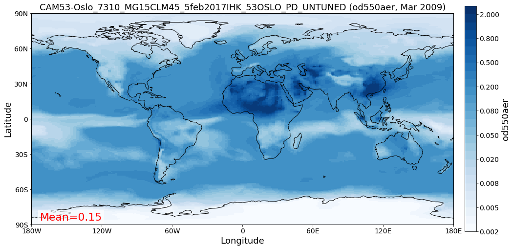
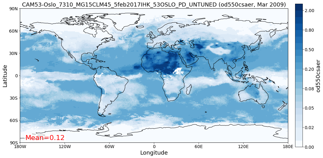
Plotting maps
Maps of individual time stamps can be plotted using the quickplot_map method.
[12]:
fig1 = od550aer.quickplot_map('2009-3-15')
fig2 = od550csaer.quickplot_map('2009-3-15')
Filtering
Regional filtering can be performed using the Filter class (cf. flowchart above).
An overview of available default regions can be accessed via:
[13]:
print(pya.region.get_all_default_region_ids())
['WORLD', 'EUROPE', 'ASIA', 'AUSTRALIA', 'CHINA', 'INDIA', 'NAFRICA', 'SAFRICA', 'SAMERICA', 'NAMERICA']
Now let’s go for north Africa. Create instance of Filter class:
[14]:
f = pya.Filter('NAFRICA')
f
[14]:
Filter([('_name', 'NAFRICA-wMOUNTAINS'),
        ('_region',
         Region NAFRICA Region([('_name', 'NAFRICA'), ('lon_range', [-20, 50]), ('lat_range', [0, 40]), ('lon_range_plot', [-20, 50]), ('lat_range_plot', [0, 40]), ('lon_ticks', None), ('lat_ticks', None)])),
        ('lon_range', [-20, 50]),
        ('lat_range', [0, 40]),
        ('alt_range', None)])
… and apply to the two data objects (this can be done by calling the filter with the corresponding data class as input parameter):
[15]:
od550aer_nafrica = f(od550aer)
od550csaer_nafrica = f(od550csaer)
Applying regional cropping in GriddedData using Filter class. Note that this does not yet include potential cropping in the vertical dimension. Coming soon...
Applying regional cropping in GriddedData using Filter class. Note that this does not yet include potential cropping in the vertical dimension. Coming soon...
Compare shapes:
[16]:
od550aer_nafrica
[16]:
pyaerocom.GriddedData
Grid data: <iris 'Cube' of Aerosol optical depth at 500nm / (1) (time: 84; latitude: 42; longitude: 57)>
[17]:
od550aer
[17]:
pyaerocom.GriddedData
Grid data: <iris 'Cube' of Aerosol optical depth at 500nm / (1) (time: 84; latitude: 192; longitude: 288)>
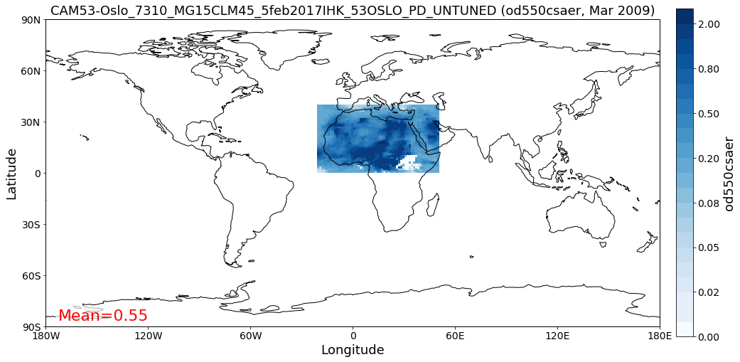
As you can see, the filtered object is reduced in the longitude and latitude dimension. Let’s plot the two new objects:
[18]:
ax1 = od550aer_nafrica.quickplot_map('2009-3-15')
ax2 = od550csaer_nafrica.quickplot_map('2009-3-15')

Filtering of time
Filtering of time is not yet included in the Filter class but can be easily performed from the GriddedData object directly. If you know the indices of the time stamps you want to crop, you can simply use numpy indexing syntax (remember that we have a 3D array containing time, latitude and lonfgitude).
Let’s say we want to filter the year 2009.
Since the time dimension corresponds the first index in the 3D data (time, lat, lon), and since we know, that we have monthly data from 2008-2010 (see above), we may use
[19]:
od550aer_nafrica_2009 = od550aer_nafrica[12:24]
od550aer_nafrica_2009.time_stamps()
[19]:
array(['2005-01-01T00:00:00.000000', '2005-02-01T00:00:00.000000',
       '2005-03-01T00:00:00.000000', '2005-04-01T00:00:00.000000',
       '2005-05-01T00:00:00.000000', '2005-06-01T00:00:00.000000',
       '2005-07-01T00:00:00.000000', '2005-08-01T00:00:00.000000',
       '2005-09-01T00:00:00.000000', '2005-10-01T00:00:00.000000',
       '2005-11-01T00:00:00.000000', '2005-12-01T00:00:00.000000'],
      dtype='datetime64[us]')
in order to extract the year 2009.
However, this methodology might not always be handy (imagine you have a 10 year dataset of 3hourly sampled data and want to extract three months in the 6th year …). In that case, you can perform the cropping using the actual timestamps (for comparibility, let’s stick to 2009 here):
[20]:
od550aer_nafrica_2009_alt = od550aer_nafrica.crop(time_range=('1-1-2009', '1-1-2010'))
od550aer_nafrica_2009.time_stamps()
[20]:
array(['2005-01-01T00:00:00.000000', '2005-02-01T00:00:00.000000',
       '2005-03-01T00:00:00.000000', '2005-04-01T00:00:00.000000',
       '2005-05-01T00:00:00.000000', '2005-06-01T00:00:00.000000',
       '2005-07-01T00:00:00.000000', '2005-08-01T00:00:00.000000',
       '2005-09-01T00:00:00.000000', '2005-10-01T00:00:00.000000',
       '2005-11-01T00:00:00.000000', '2005-12-01T00:00:00.000000'],
      dtype='datetime64[us]')
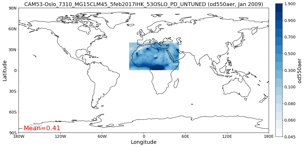
Data aggregation
Let’s say we want to compute yearly means for each of the 3 years. In this case we can simply call the downscale_time method:
[21]:
od550aer_nafrica.downscale_time('yearly')
od550aer_nafrica.quickplot_map('2009')
This method is deprecated. Please use new name resample_time
[21]:

Note: seasonal aggregation is not yet implemented in pyaerocom but will follow soon.
In the following section the reading of ungridded data is illustrated based on the example of AERONET version 3 (level 2) data. The test dataset contains a randomly picked subset of 100 Aeronet stations. Aeronet provides different products,
Reading of and working with ungridded data (ReadUngridded and UngriddedData classes)
Ungridded data in pyaerocom refers to data that is available in the form of files per station and that is not sampled in a manner that it would make sense to translate into a rgular gridded format such as the previously introduced GriddedData class.
Data from the AERONET network (that is introduced in the following), for instance, is provided in the form of column seperated text files per measurement station, where columns correspond to different variables and data rows to individual time stamps. Needless to say that the time stamps (or the covered periods) vary from station to station.
The basic workflow for reading of ungridded data, such as Aeronet data, is very similar to the reading of gridded data (comprising a reading class that handles a query and returns a data class, here UngriddedData (see also flow chart above).
Before we can continue with the data import, some things need to be said related to the caching of UngriddedData objects.
Caching of UngriddedData
Reading of ungridded data is often rather time-consuming. Therefore, pyaerocom uses a caching strategy that stores loaded instances of the UngriddedData class as pickle files in a cache directory (illustrated in the left hand side of the flowchart shown above). The loaction of the cache directory can be accessed via:
[22]:
pya.const.CACHEDIR
[22]:
'/home/jonasg/MyPyaerocom/_cache/jonasg'
You may change this directory if required.
[23]:
print('Caching is active? {}'.format(pya.const.CACHING))
Caching is active? True
Deactivate / Activate caching
[24]:
pya.const.CACHING = False
[25]:
pya.const.CACHING = True
Note: if caching is active, make sure you have enough disk quota or change location where the files are stored.
Read Aeronet Sun v3 level 2 data
As illustrated in the flowchart above, ungridded observation data can be imported using the ReadUngridded class. The reading class requires an ID for the observation network that is supposed to be read. Let’s find the right ID for these data:
[26]:
pya.browse_database('Aeronet*V3*Lev2*')
Dataset name: AeronetSunV3Lev2.daily
Data directory: /lustre/storeA/project/aerocom/aerocom1/AEROCOM_OBSDATA/AeronetSunV3Lev2.0.daily/renamed
Supported variables: ['od340aer', 'od440aer', 'od500aer', 'od870aer', 'ang4487aer', 'ang4487aer_calc', 'od550aer']
Last revision: 20190920

Dataset name: AeronetSunV3Lev2.AP
Data directory: /lustre/storeA/project/aerocom/aerocom1/AEROCOM_OBSDATA/AeronetSunV3Lev2.0.AP/renamed
Supported variables: ['od340aer', 'od440aer', 'od500aer', 'od870aer', 'ang4487aer', 'ang4487aer_calc', 'od550aer']
Last revision: 20190511

Dataset name: AeronetSDAV3Lev2.daily
Data directory: /lustre/storeA/project/aerocom/aerocom1/AEROCOM_OBSDATA/Aeronet.SDA.V3L2.0.daily/renamed
Supported variables: ['od500gt1aer', 'od500lt1aer', 'od500aer', 'ang4487aer', 'od550aer', 'od550gt1aer', 'od550lt1aer']
Last revision: 20190920
Reading failed for AeronetSDAV3Lev2.AP. Error: NetworkNotImplemented('No reading class available yet for dataset AeronetSDAV3Lev2.AP')

Dataset name: AeronetInvV3Lev2.daily
Data directory: /lustre/storeA/project/aerocom/aerocom1/AEROCOM_OBSDATA/Aeronet.Inv.V3L2.0.daily/renamed
Supported variables: ['abs440aer', 'angabs4487aer', 'od440aer', 'ang4487aer', 'abs550aer', 'od550aer']
Last revision: 20190914
It found one match and the dataset ID is AeronetSunV3Lev2.daily. It also tells us what variables can be loaded via the interface.
Note: You can safely ignore all the warnings in the output. These are due to the fact that the testdata set does not contain all observation networks that are available in the AEROCOM database.
[27]:
obs_reader = pya.io.ReadUngridded('AeronetSunV3Lev2.daily')
print(obs_reader)
Dataset name: AeronetSunV3Lev2.daily
Data directory: /lustre/storeA/project/aerocom/aerocom1/AEROCOM_OBSDATA/AeronetSunV3Lev2.0.daily/renamed
Supported variables: ['od340aer', 'od440aer', 'od500aer', 'od870aer', 'ang4487aer', 'ang4487aer_calc', 'od550aer']
Last revision: 20190920
Let’s read the data (you can read a single or multiple variables at the same time). For now, we only read the AOD at 550 nm:
[28]:
aeronet_data = obs_reader.read(vars_to_retrieve='od550aer')
type(aeronet_data) #displays data type
[28]:
pyaerocom.ungriddeddata.UngriddedData
As you can see, the data object is of type UngriddedData. Like the GriddedData object, also the UngriddedData class has an informative string representation (that can be printed):
[29]:
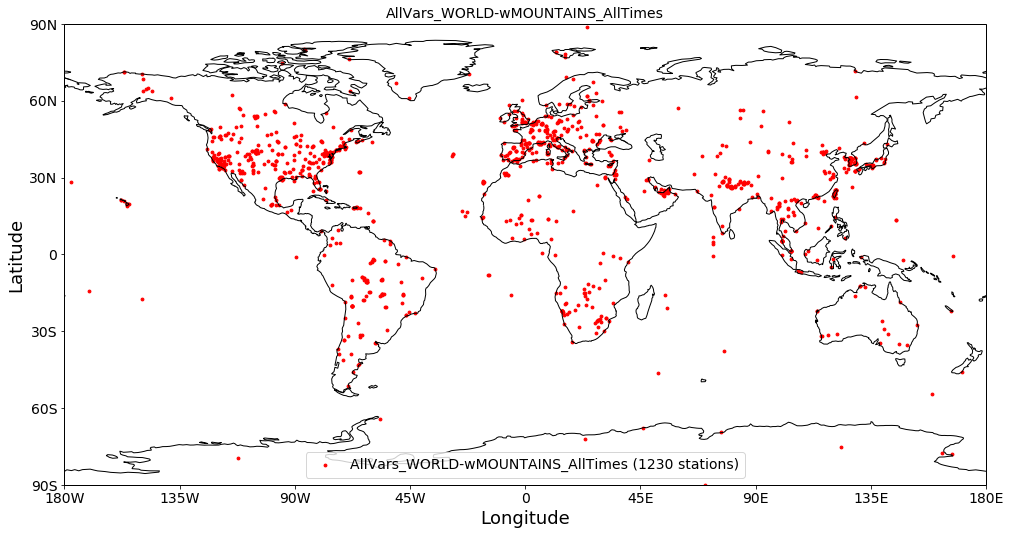
print(aeronet_data)
Pyaerocom UngriddedData
-----------------------
Contains networks: ['AeronetSunV3Lev2.daily']
Contains variables: ['od550aer']
Contains instruments: ['sun_photometer']
Total no. of meta-blocks: 1230
Filters that were applied:
 Filter time log: 20191002122003
        Created od550aer single var object from multivar UngriddedData instance
Plot all station coordinates
[30]:
aeronet_data.plot_station_coordinates();
Access of individual stations
Get all station names:
[31]:
all_station_names = aeronet_data.unique_station_names
all_station_names[:10]  #displays first 10 stations
[31]:
['AAOT',
 'AOE_Baotou',
 'ARM_Ascension_Is',
 'ARM_Barnstable_MA',
 'ARM_Cordoba',
 'ARM_Darwin',
 'ARM_Gan_Island',
 'ARM_Graciosa',
 'ARM_Highlands_MA',
 'ARM_HyytialaFinland']
For instance, to access the data for the city of Leipzig, Germany, you can use square brackets with the station name of Leipzig:
[32]:
station_data = aeronet_data['Leipzig'] # this is fully equivalent with aeronet_data.to_station_data('Leipzig')
type(station_data)
[32]:
pyaerocom.stationdata.StationData
As you can see, the returned object is of type StationData, which is one further data format of pyaerocom (note that this is not displayed in the simplified flowchart above). StationData may be useful for individual stations and is an extended Python dictionary (if you are familiar with Python).
You may print it to see what is in there:
[33]:
print(station_data)
Pyaerocom StationData
---------------------
var_info (BrowseDict):
  od550aer (OrderedDict):
    units: 1
    overlap: False
    ts_type: daily
    apply_constraints: False
    min_num_obs: None
station_coords (dict):
  latitude: 51.352500000000006
  longitude: 12.435277999999998
  altitude: 125.0
data_err (BrowseDict): <empty_dict>
overlap (BrowseDict): <empty_dict>
data_flagged (BrowseDict): <empty_dict>
filename: None
station_id: None
station_name: Leipzig
instrument_name: sun_photometer
PI: Brent_Holben
country: None
ts_type: daily
latitude: 51.352500000000006
longitude: 12.435277999999998
altitude: 125.0
data_id: AeronetSunV3Lev2.daily
dataset_name: None
data_product: None
data_version: None
data_level: None
revision_date: None
website: None
ts_type_src: daily
stat_merge_pref_attr: None
data_revision: 20190920

Data arrays
.................
dtime (ndarray, 6363 items): [2001-05-21T00:00:00.000000000, 2001-05-22T00:00:00.000000000, ..., 2018-10-20T00:00:00.000000000, 2018-10-21T00:00:00.000000000]
Pandas Series
.................
od550aer (Series, 6363 items)
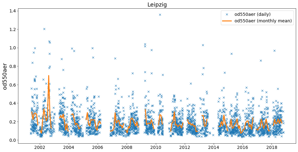
As you can see, this station contains a time-series of the AOD at 550 nm. If you like, you can plot this time-series:
[34]:
ax = station_data.insert_nans_timeseries('od550aer').plot_timeseries('od550aer', marker='x', ls='none')
station_data.plot_timeseries('od550aer', freq='monthly', marker=' ', ls='-', lw=3, ax=ax)
[34]:
<matplotlib.axes._subplots.AxesSubplot at 0x7f2c2061e3c8>
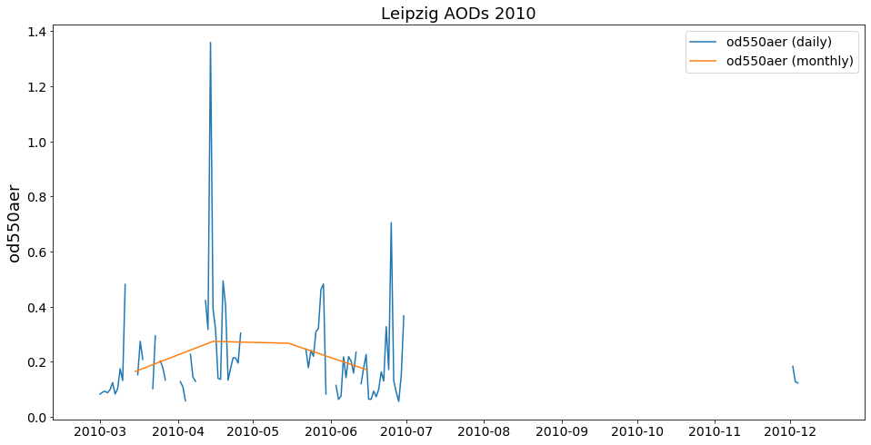
You can also retrieve the StationData with specifying more constraints using to_station_data (e.g. in monthly resolution and only for the year 2010). And you can overlay different curves, by passing the axes instance returned by the plotting method:
[35]:
ax=aeronet_data.to_station_data('Leipzig',
                                start=2010,
                                freq='daily').plot_timeseries('od550aer')

ax=aeronet_data.to_station_data('Leipzig',
                                start=2010,
                                freq='monthly').plot_timeseries('od550aer', ax=ax)
ax.legend()
ax.set_title('Leipzig AODs 2010')
[35]:
Text(0.5, 1.0, 'Leipzig AODs 2010')
You can also plot the time-series directly
For instance, if you want to do an air-quality check for you next bouldering trip, you may call:
[36]:
ts = aeronet_data.to_station_data('Fontainebleau', 'od550aer', 2006, None, 'monthly')
ts
[36]:
StationData([('dtime',
              array(['2006-01-15T00:00:00.000000000', '2006-02-15T00:00:00.000000000',
                     '2006-03-15T00:00:00.000000000', '2006-04-15T00:00:00.000000000',
                     '2006-05-15T00:00:00.000000000', '2006-06-15T00:00:00.000000000',
                     '2006-07-15T00:00:00.000000000', '2006-08-15T00:00:00.000000000',
                     '2006-09-15T00:00:00.000000000', '2006-10-15T00:00:00.000000000',
                     '2006-11-15T00:00:00.000000000', '2006-12-15T00:00:00.000000000'],
                    dtype='datetime64[ns]')),
             ('var_info',
              BrowseDict([('od550aer',
                           OrderedDict([('units', '1'),
                                        ('overlap', False),
                                        ('ts_type', 'monthly'),
                                        ('apply_constraints', True),
                                        ('min_num_obs',
                                         {'yearly': {'monthly': 3},
                                          'monthly': {'daily': 7},
                                          'daily': {'hourly': 6},
                                          'hourly': {'minutely': 15}})]))])),
             ('station_coords',
              {'latitude': 48.406666999999985,
               'longitude': 2.6802780000000004,
               'altitude': 85.0}),
             ('data_err', BrowseDict()),
             ('overlap', BrowseDict()),
             ('data_flagged', BrowseDict()),
             ('filename', None),
             ('station_id', None),
             ('station_name', 'Fontainebleau'),
             ('instrument_name', 'sun_photometer'),
             ('PI', 'Brent_Holben'),
             ('country', None),
             ('ts_type', 'monthly'),
             ('latitude', 48.406666999999985),
             ('longitude', 2.6802780000000004),
             ('altitude', 85.0),
             ('data_id', 'AeronetSunV3Lev2.daily'),
             ('dataset_name', None),
             ('data_product', None),
             ('data_version', None),
             ('data_level', None),
             ('revision_date', None),
             ('website', None),
             ('ts_type_src', 'daily'),
             ('stat_merge_pref_attr', None),
             ('data_revision', '20190920'),
             ('od550aer', 2006-01-15    0.176742
              2006-02-15         NaN
              2006-03-15    0.252403
              2006-04-15    0.195318
              2006-05-15    0.215357
              2006-06-15    0.195586
              2006-07-15    0.224991
              2006-08-15    0.131814
              2006-09-15    0.151338
              2006-10-15    0.141222
              2006-11-15    0.088815
              2006-12-15         NaN
              Name: mean, dtype: float64)])
[37]:
aeronet_data.plot_station_timeseries('Fontainebleau', 'od550aer', ts_type='monthly',
                                     start=2006).set_title('AOD in Fontainebleau, 2006')
[37]:
Text(0.5, 1.0, 'AOD in Fontainebleau, 2006')
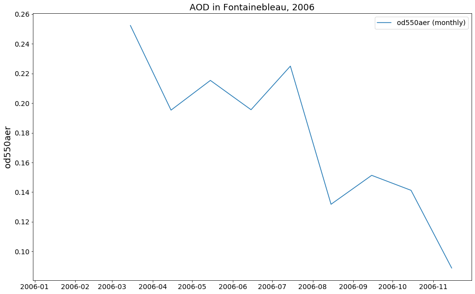
Seems like November is a good time (maybe a bit rainy though)
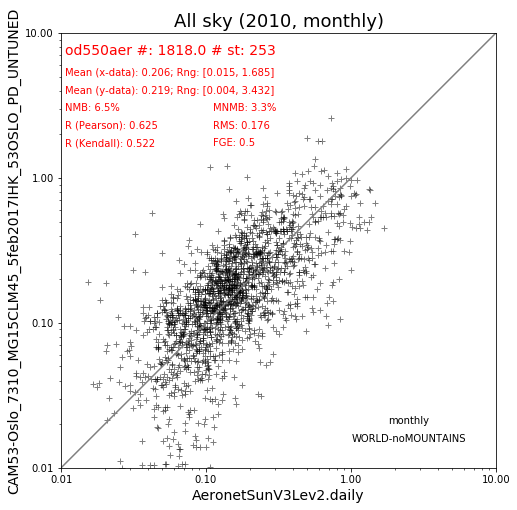
Colocation of model and obsdata
Now that we have different data objects loaded we can continue with colocation. In the following, both the all-sky and the clear-sky data from CAM53-Oslo will be colocated with the subset of Aeronet stations that we just loaded.
The colocation will be performed for the year of 2010 and two scatter plots will be created.
You have also the option to apply a certain filter when colocating using a valid filter name. Here, we use global data and exclude mountain sides.
[38]:
col_all_sky_glob = pya.colocation.colocate_gridded_ungridded(od550aer, aeronet_data,
                                                                ts_type='monthly',
                                                                start=2010,
                                                                filter_name='WORLD-noMOUNTAINS')
type(col_all_sky_glob)
Setting od550aer outlier lower lim: -1.00
Setting od550aer outlier upper lim: 10.00
Interpolating data of shape (12, 192, 288). This may take a while.
Successfully interpolated cube
[38]:
pyaerocom.colocateddata.ColocatedData
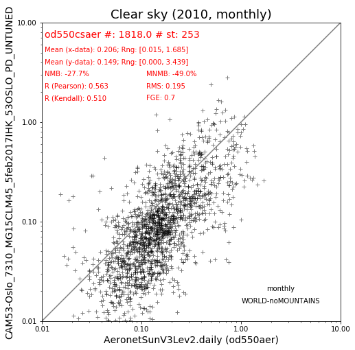
Let’s do the same for the clear-sky data.
[39]:
col_clear_sky_glob = pya.colocation.colocate_gridded_ungridded(od550csaer, aeronet_data,
                                                                  ts_type='monthly',
                                                                  start=2010,
                                                                  filter_name='WORLD-noMOUNTAINS')
type(col_clear_sky_glob)
Setting od550aer outlier lower lim: -1.00
Setting od550aer outlier upper lim: 10.00
Interpolating data of shape (12, 192, 288). This may take a while.
Successfully interpolated cube
[39]:
pyaerocom.colocateddata.ColocatedData
[40]:
ax1 = col_all_sky_glob.plot_scatter()
ax1.set_title('All sky (2010, monthly)');
[41]:
ax2 = col_clear_sky_glob.plot_scatter()
ax2.set_title('Clear sky (2010, monthly)');
… or for EUROPE:
[42]:
pya.colocation.colocate_gridded_ungridded(od550aer, aeronet_data,
                                          ts_type='monthly',
                                          start=2010,
                                          filter_name='EUROPE-noMOUNTAINS').plot_scatter();
Setting od550aer outlier lower lim: -1.00
Setting od550aer outlier upper lim: 10.00
Interpolating data of shape (12, 192, 288). This may take a while.
Successfully interpolated cube

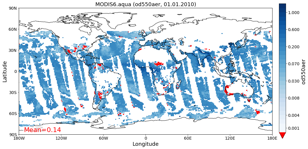
Colocation with satellite AODs from MODIS
[43]:
sat_data = pya.io.ReadGridded('MODIS6.aqua').read_var('od550aer', start=2010)
sat_data.quickplot_map(vmin=.001, vmax=3, c_under='r');
Overwriting unit unknown in cube od550aer with value "1"
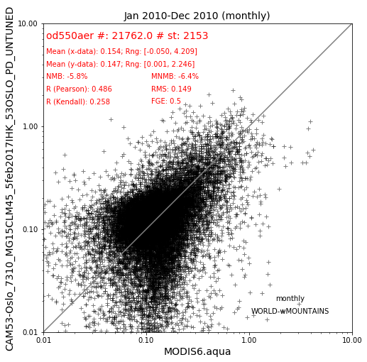
Colocation is straight forward as shown below. The data will be regridded to 5x5 degrees resolution during the colocation.
[44]:
col_modis_monthly = pya.colocation.colocate_gridded_gridded(gridded_data=od550aer,
                                                            gridded_data_ref=sat_data,
                                                            ts_type='monthly',
                                                            regrid_res_deg=5,
                                                            remove_outliers=True,
                                                            harmonise_units=False)
Interpolating data of shape (365, 180, 360). This may take a while.
Successfully interpolated cube
Setting od550aer outlier lower lim: -1.00
Setting od550aer outlier upper lim: 10.00
[45]:
col_modis_monthly.plot_scatter()
[45]:
<matplotlib.axes._subplots.AxesSubplot at 0x7f2c1049a198>
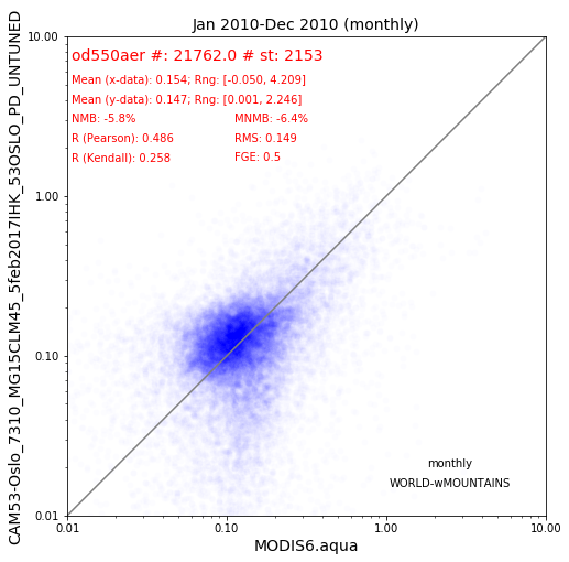
You may also change the plot style, to adapt better to the large amount of data points here in these satellite products:
[46]:
col_modis_monthly.plot_scatter(ms=6, marker='o',mec='none', color='b', alpha=0.01)
[46]:
<matplotlib.axes._subplots.AxesSubplot at 0x7f2c10614908>
Remark on the ColocatedData object
The ColocatedData object has not many features and methods implemented yet. But it builds a good basis for further analysis using features of the underlying data-structure, which is an instance of the xarray.DataArray class and can be accessed via the data attribute if the ColocatedData object:
[47]:
arr = col_all_sky_glob.data
type(arr)
[47]:
xarray.core.dataarray.DataArray
You may want to read more about it here.