Introduction into the UngriddedData class and the StationData class
This notebook introduces 2 of the most relevant data objects that exist in pyaerocom:
``UngriddedData``
Designed to hold a whole database of observations, that is, timeseries data for multiple variables from multiple stations around the globe.
Supports also 3D variables (e.g. timeseries of lidar profiles).
Usually, one instance of this data object contains a single network, but it can also contain more than one network.
``StationData``
Data object that contains data from a single station.
Includes metadata and variable timeseries data.
Arbitrary number of variables supported.
NOTE
This notebook is currently under development and gives only a brief and incomplete introduction into the two data objects.
The UngriddedData object
The first part of the tutorial shows some features of the UngriddedData object.
Import the UngriddedData object that was created in the previous tutorial
[1]:
import pyaerocom as pya
# read the data from the storage
%store -r data

data
Initating pyaerocom configuration
Checking database access...
Checking access to: /lustre/storeA
Access to lustre database: True
Init data paths for lustre
Expired time: 0.016 s
[1]:
UngriddedData <networks: ['AeronetSunV3Lev2.daily']; vars: ['od550aer']; instruments: ['sun_photometer'];No. of stations: 1230
Create an overview map of all stations
Before digging a little deeper into the UngriddedData object, let’s get an overview of the bigger picture:
[2]:
# plots all stations as red dots
ax = data.plot_station_coordinates(markersize=12, color='r')

# add all stations that contain AOD data in 2010 in green
ax = data.plot_station_coordinates(var_name='od550aer',
                                   start=2010,
                                   stop=2011, color='lime', ax=ax)
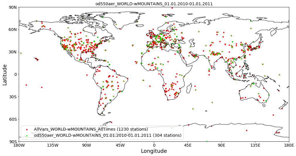
As you can see, you can specify additional input parameters, e.g. to display only stations that contain variable data or to specify a time interval.
In any case, it is always good to know about the help function:
[3]:
help(data.plot_station_coordinates)
Help on method plot_station_coordinates in module pyaerocom.ungriddeddata:

plot_station_coordinates(var_name=None, filter_name=None, start=None, stop=None, ts_type=None, color='r', marker='o', markersize=8, fontsize_base=10, **kwargs) method of pyaerocom.ungriddeddata.UngriddedData instance
    Plot station coordinates on a map

    All input parameters are optional and may be used to add constraints
    related to which stations are plotted. Default is all stations of all
    times.

    Parameters
    ----------

    var_name : :obj:`str`, optional
        name of variable to be retrieved
    filter_name : :obj:`str`, optional
        name of filter (e.g. EUROPE-noMOUNTAINS)
    start
        start time (optional)
    stop
        stop time (optional). If start time is provided and stop time not,
        then only the corresponding year inferred from start time will be
        considered
    ts_type : :obj:`str`, optional
        temporal resolution
    color : str
        color of stations on map
    marker : str
        marker type of stations
    markersize : int
        size of station markers
    fontsize_base : int
        basic fontsize
    **kwargs
        Addifional keyword args passed to
        :func:`pyaerocom.plot.plot_coordinates`

    Returns
    -------
    axes
        matplotlib axes instance
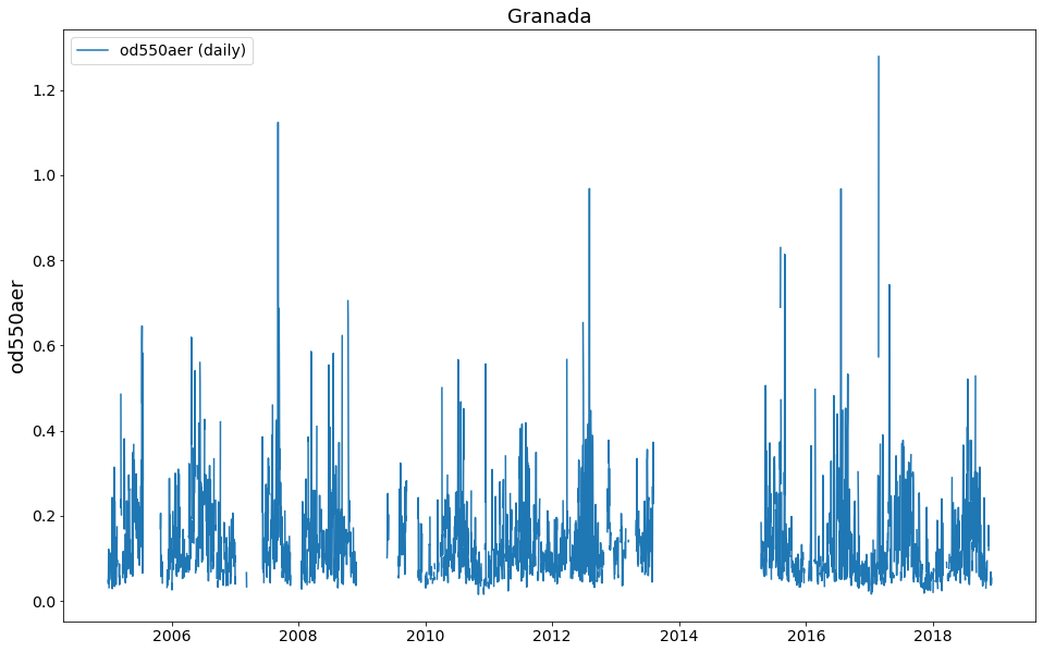
Quicklook plotting of station timeseries
Time series of individual stations can be plotted as follows:
[4]:
data.plot_station_timeseries(station_name='Granada', var_name='od550aer');
Access metadata of the data files that were read
Look into the metadata of the different files. Metadata can be accessed via the metadata attribute, and there is one metadatadictionary for each file that was read:
[5]:
len(data.metadata)
[5]:
1230
Access metadata of first file (index 0):
[6]:
data.metadata[0]
[6]:
{'var_info': OrderedDict([('od550aer', OrderedDict([('units', '1')]))]),
 'latitude': 45.3139,
 'longitude': 12.508299999999998,
 'altitude': 10.0,
 'station_name': 'AAOT',
 'PI': 'Brent_Holben',
 'ts_type': 'daily',
 'data_id': 'AeronetSunV3Lev2.daily',
 'variables': ['od550aer'],
 'instrument_name': 'sun_photometer',
 'data_revision': '20190920'}
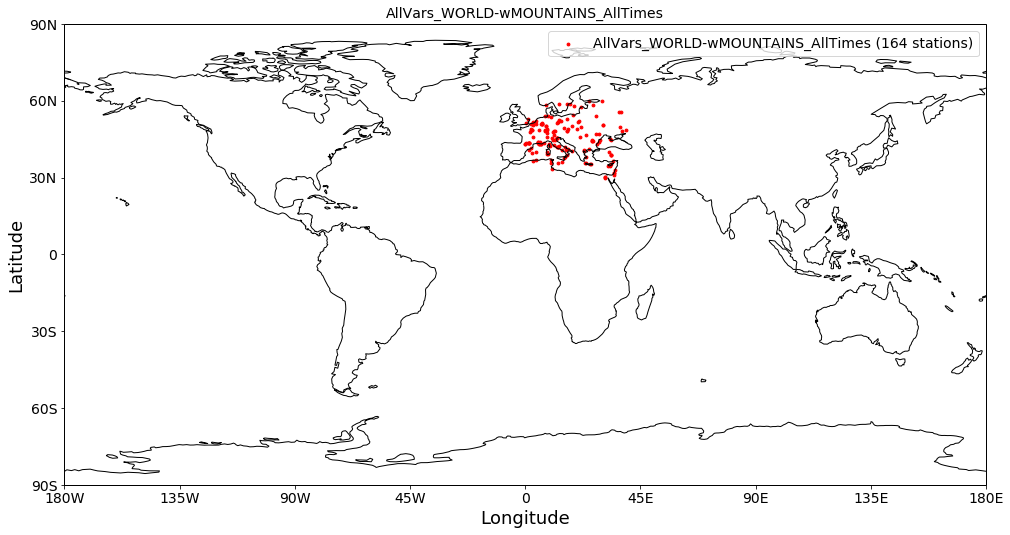
Filtering of the data
So far, you can filter UngriddedData objects by common metadata attributes. For instance:
[7]:
subset = data.filter_by_meta(latitude=(30, 60), longitude=(0, 45), altitude=(0, 1000))
print(subset)
Pyaerocom UngriddedData
-----------------------
Contains networks: ['AeronetSunV3Lev2.daily']
Contains variables: ['od550aer']
Contains instruments: ['sun_photometer']
Total no. of meta-blocks: 164
Filters that were applied:
 Filter time log: 20191002122003
        Created od550aer single var object from multivar UngriddedData instance
 Filter time log: 20191003180107
        latitude: (30, 60)
        longitude: (0, 45)
        altitude: (0, 1000)
[8]:
subset.plot_station_coordinates();
Other attributes that may be useful
Access all station names and print the first 4:
[9]:
stat_names = data.station_name
print(stat_names[:4])
['AAOT', 'AOE_Baotou', 'ARM_Ascension_Is', 'ARM_Barnstable_MA']
Essentially, what data.station_name does is, it iterates over all metadata-dictionaries (that are stored in data.metadata, and are organised per file that was read) and extracts the station_name attribute and appends it to a list which is then returned by the method.
Hence, the list of station names corresponds to the list of metadata-blocks / files that are stored in the data object:
[10]:
len(stat_names)
[10]:
1230
In a similar manner, you can access coordinates latitude, longitude and altitude arrays for all files.
[11]:
lons = data.longitude
lons[:4]
[11]:
[12.508299999999998,
 109.62879999999998,
 -14.349805999999996,
 -70.29006100000001]
[12]:
lats = data.latitude
lats[:4]
[12]:
[45.3139, 40.851699999999994, -7.966963999999998, 41.669588999999995]
[13]:
alts = data.altitude
alts[:4]
[13]:
[10.0, 1314.0, 341.0, 15.0]
List of unique station names
As mentioned earlier, some databases provide more than one data file per station. Since the ungridded reading (see previous) tutorial is done per data file, this means that their can be more than one metadata-block per station (not the case here, though). In any case, you can get a list of unique station names using:
[14]:
unique_names = data.unique_station_names
unique_names[:4]
[14]:
['AAOT', 'AOE_Baotou', 'ARM_Ascension_Is', 'ARM_Barnstable_MA']
StationData: Access the data from individual stations
As you could see above the metadata dictionaries in the UngriddedData class for each file do only contain the associated metadata. For the sake of performance the actual data arrays are all stored in one big 2D numpy array (which does not need to bother you too much) which is accessible in the _data attribute of the UngriddedData object (if you like to dive into it).
In most cases that concern model evaluation, the observation data is analysed station-by-station. For this purpose the StationData class was designed, which is introduced below.
Starting from an instance of the UngriddedData object, the individual station data (i.e. time series of one or more variables + metadata) can be accessed using the method:
or using the square brackets [] which is equivalent to the former as it is only a wrapper for to_station_data. This meants, calling
UngriddedData[0]
will give you the same output as
UngriddedData.to_station_data[0]
that is, the data associated with the first file that was read (i.e. the first metadata-block in the object) into the UngriddedData object (see previous tutorial for details regarding the reading of ungridded observation networks).
To specify the station, you can either use the metadata index of the corresponding data file (meta_idx=9, for 10th file) or you can specify the station name or a wildcard specifying the station name.
The method returns a pyaerocom.StationData object, which is a dictionary-like object which contains data vectors and time-stamps as well as metadata.
Below we will illustrate the several options to access station data (and show that they contain the same data):
Option 1. Get station data using the corresponding metadata indices that match the station name
Find index (or indices) that match the station name:
[15]:
index = data.find_station_meta_indices('Granada')
index
[15]:
[497]
The result shows that there is one file that matches this station name (as we would expect for AERONET data) and the corresponding metadata index is 488.
To access the data, you can use the method to_station_data. It helps to have a look into the options of this method:
[16]:
help(data.to_station_data)
Help on method to_station_data in module pyaerocom.ungriddeddata:

to_station_data(meta_idx, vars_to_convert=None, start=None, stop=None, freq=None, merge_if_multi=True, merge_pref_attr=None, merge_sort_by_largest=True, insert_nans=False, **kwargs) method of pyaerocom.ungriddeddata.UngriddedData instance
    Convert data from one station to :class:`StationData`

    Todo
    ----
    - Review for retrieval of profile data (e.g. Lidar data)

    Parameters
    ----------
    meta_idx : float
        index of station or name of station.
    vars_to_convert : :obj:`list` or :obj:`str`, optional
        variables that are supposed to be converted. If None, use all
        variables that are available for this station
    start
        start time, optional (if not None, input must be convertible into
        pandas.Timestamp)
    stop
        stop time, optional (if not None, input must be convertible into
        pandas.Timestamp)
    freq : str
        pandas frequency string (e.g. 'D' for daily, 'M' for month end) or
        valid pyaerocom ts_type
    merge_if_multi : bool
        if True and if data request results in multiple instances of
        StationData objects, then these are attempted to be merged into one
        :class:`StationData` object using :func:`merge_station_data`
    merge_pref_attr
        only relevant for merging of multiple matches: preferred attribute
        that is used to sort the individual StationData objects by relevance.
        Needs to be available in each of the individual StationData objects.
        For details cf. :attr:`pref_attr` in docstring of
        :func:`merge_station_data`. Example could be `revision_date`. If
        None, then the stations will be sorted based on the number of
        available data points (if :attr:`merge_sort_by_largest` is True,
        which is default).
    merge_sort_by_largest : bool
        only relevant for merging of multiple matches: cf. prev. attr. and
        docstring of :func:`merge_station_data` method.
    insert_nans : bool
        if True, then the retrieved :class:`StationData` objects are filled
        with NaNs

    Returns
    -------
    StationData or list
        StationData object(s) containing results. list is only returned if
        input for meta_idx is station name and multiple matches are
        detected for that station (e.g. data from different instruments),
        else single instance of StationData. All variable time series are
        inserted as pandas Series
So the first input argument takes either the metadata index, or the name of the station. Here we use the metadata index option using the index that we just retrieved:
[17]:
granada_opt1 = data.to_station_data(meta_idx=index[0], insert_nans=True)
type(granada_opt1)
[17]:
pyaerocom.stationdata.StationData
The returned data type is an instance of the pyaerocom.StationData class.
NOTE: if there is more than one index match for one station (i.e. data.find_station_meta_indices('Granada') returns more than one match), then, using Option 1, you would need to call to_station_data for each of the index matches. Alternatively you could use either of the following methods, which automatically merge the individual StationData objects into one, in case of multiple matches for that station name.
Let’s have a quick look at the StationData object (it is a dictionary-like object and simple to use):
Option 2: Retrieve station data using the station name directly
[18]:
granada_opt2 = data.to_station_data('Granada', insert_nans=True)
Other than option 1, in case of multiple meta-index matches, this method automatically merges the individual data objects.
Option 3: Use […] notation
This is a wrapper for the method to_station_data so you may use meta-index or station name for access.
[19]:
granada_opt3_1 = data[index[0]]
granada_opt3_2 = data['Granada']
Let’s have a look if the data objects are really the same (by plotting the AOD timeseries for the 4 different options):
[20]:
ax = granada_opt1.plot_timeseries('od550aer', lw=3, label='Option 1', tit='Method: UngriddedData.to_station_data()')
granada_opt2.plot_timeseries('od550aer', ls='--', lw=1, label='Option 2',ax=ax)

# plot the results from the [] access option into a new figure (don't pass ax)
ax = granada_opt3_1.plot_timeseries('od550aer', lw=3, label='Option 3.1 (using meta-index)',
                                    tit='Method: UngriddedData[]')
granada_opt3_2.plot_timeseries('od550aer', ls='--', lw=1, label='Option 3.2 (using station name)',ax=ax)
[20]:
<matplotlib.axes._subplots.AxesSubplot at 0x7f3a66706a20>
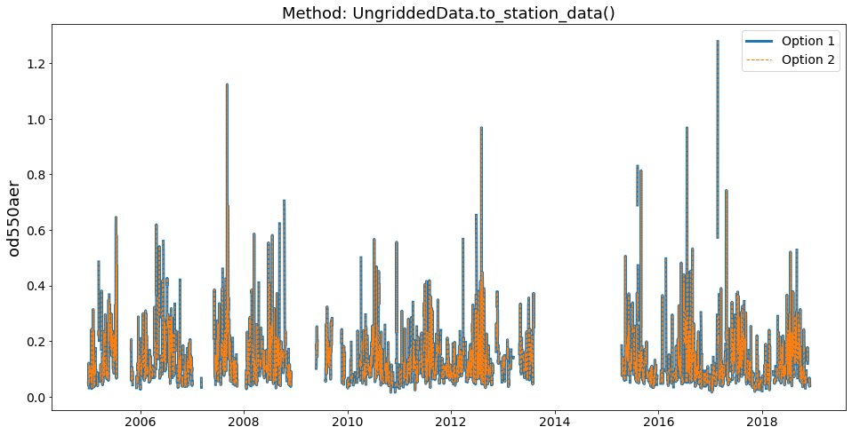
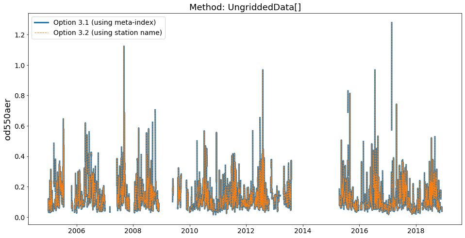
Looks good. Let’s explore the StationData object a little more (you can print it and it will get you a nice overview):
[21]:
print(granada_opt1)
Pyaerocom StationData
---------------------
var_info (BrowseDict):
  od550aer (OrderedDict):
    units: 1
    overlap: False
    ts_type: daily
    apply_constraints: False
    min_num_obs: None
station_coords (dict):
  latitude: 37.163999999999994
  longitude: -3.6049999999999995
  altitude: 680.0
data_err (BrowseDict): <empty_dict>
overlap (BrowseDict): <empty_dict>
data_flagged (BrowseDict): <empty_dict>
filename: None
station_id: None
station_name: Granada
instrument_name: sun_photometer
PI: Brent_Holben
country: None
ts_type: daily
latitude: 37.163999999999994
longitude: -3.6049999999999995
altitude: 680.0
data_id: AeronetSunV3Lev2.daily
dataset_name: None
data_product: None
data_version: None
data_level: None
revision_date: None
website: None
ts_type_src: daily
stat_merge_pref_attr: None
data_revision: 20190920

Data arrays
.................
dtime (ndarray, 5087 items): [2004-12-30T00:00:00.000000000, 2004-12-31T00:00:00.000000000, ..., 2018-12-02T00:00:00.000000000, 2018-12-03T00:00:00.000000000]
Pandas Series
.................
od550aer (Series, 5087 items)
You can see that the StationData object contains both metadata (e.g. PI) and data vectors which can be either 1D numpy arrays or python lists (e.g. dtime) or pandas.Series objects (e.g. variable od550aer). All attributes can be accessed and manipulated either using dictionary style access (i.e. [] notation), or using the . operator.
Here some examples:
[22]:
# get longitude using "[]" notation
granada_opt1['longitude']
[22]:
-3.6049999999999995
[23]:
# get longitude using "." notation
granada_opt1.longitude
[23]:
-3.6049999999999995
[24]:
# assign longitude using "." notation and display new value (again using "[]" notation)
granada_opt1.longitude = 42
granada_opt1['longitude']
[24]:
42
[25]:
granada_opt1['station_name']
[25]:
'Granada'
Get station name:
[26]:
granada_opt1.station_name
[26]:
'Granada'
Small detour through the pandas world
As you can see in the output above, the time-series data in the StationData object is an instance of the pandas.Series class.
[27]:
aod_data = granada_opt1.od550aer
type(aod_data)
[27]:
pandas.core.series.Series
NOTE: pyaerocom relies on pandas, so if you are not familiar with the pandas library, it is a good advice to make yourself familiar with it (especially if you are interested in timeseries analysis). See here for a short introduction into pandas.
Anyways, you should know about the 2 basic datatypes of pandas which are:
Both objects are very similar in their handling and the Series class can be imagined as a single column of the Dataframe object which is a table-like object that has columns (e.g. variables) and rows (e.g. time-stamps). It is hence, easy to go back and forth between the two objects.
Anyways, here is some examples what you can do with an instance of the pandas.Series object that we just accessed from the pyaerocom.StationData object from Granada (and which we named aod_data).
First, you can get a basic clue about the data by using the describe method:
[28]:
aod_data.describe()
[28]:
count    3010.000000
mean        0.137759
std         0.103330
min         0.015534
25%         0.070969
50%         0.108200
75%         0.171291
max         1.278507
dtype: float64
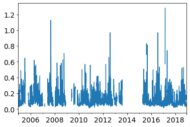
Second, you may plot it:
[29]:
aod_data.plot();
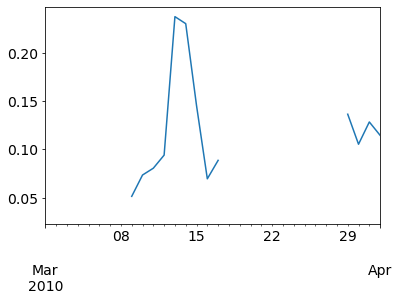
Third, you may extract subsets using fancy indexing:
[30]:
aod_data_march2010 = aod_data['2010-3-1':'2010-4-1']
aod_data_march2010.plot();
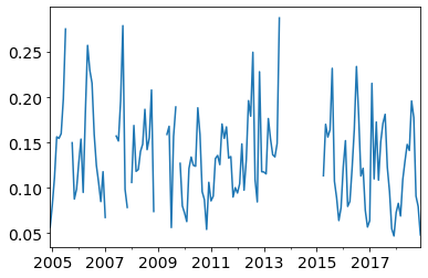
Or fourth, resample to another frequency:
[31]:
aod_data_monthly = aod_data.resample('M', 'mean')
aod_data_monthly.plot();
Or fifth, resample to lower frequency, but require a minimum number of observations per period:
[32]:
monthly_with_count = aod_data.resample('M').agg(['mean', 'count'])
monthly_with_count.head()
[32]:
| mean | count | |
|---|---|---|
| 2004-12-31 | 0.056462 | 1 |
| 2005-01-31 | 0.081300 | 28 |
| 2005-02-28 | 0.111567 | 24 |
| 2005-03-31 | 0.156312 | 17 |
| 2005-04-30 | 0.154527 | 26 |
Now, here you see an example, where pandas automatically converted our Series (which is single variable) to a DataFrame (which is a table), since we told the resampler above, to aggregate monthly mean and monthly count.
Now let’s say we require at least 15 observations (here, days, since our original dataset is in daily resolution) per month:
[33]:
invalid_mask = monthly_with_count['count'] < 15
monthly_with_count['mean'][invalid_mask] = np.nan
aod_monthly_min15d = monthly_with_count['mean']
aod_monthly_min15d.head()
[33]:
2004-12-31         NaN
2005-01-31    0.081300
2005-02-28    0.111567
2005-03-31    0.156312
2005-04-30    0.154527
Freq: M, Name: mean, dtype: float64
Now plot both the monthly timeseries from above without constraint and the one with constraint:
[34]:
ax = aod_data_monthly.plot(label='Monthly without constraint', lw=3, figsize=(14,6))
aod_monthly_min15d.plot(ax=ax, style='x-', label='Monthly (at least 15 days per month)')
ax.legend();
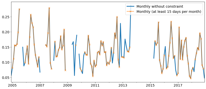
As you can see, there is quite some months missing when applying the filter.
You may also be intersted in a climatology:
[35]:
aod_monthly_climatology = aod_data_monthly.groupby(aod_data_monthly.index.month).mean()
aod_monthly_climatology
[35]:
1     0.091885
2     0.125760
3     0.114174
4     0.132566
5     0.146915
6     0.164997
7     0.174380
8     0.192138
9     0.146022
10    0.115006
11    0.091344
12    0.082346
dtype: float64
And do the same for the monthly data with minimum 15 days per month that we created above:
[36]:
aod_monthly_climatology_min15d = aod_monthly_min15d.groupby(aod_monthly_min15d.index.month).mean()
aod_monthly_climatology_min15d
[36]:
1     0.093066
2     0.130359
3     0.119908
4     0.136720
5     0.145820
6     0.164751
7     0.184243
8     0.183453
9     0.141699
10    0.111532
11    0.072294
12    0.089056
Name: mean, dtype: float64
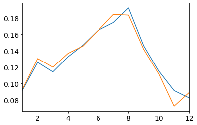
[37]:
ax = aod_monthly_climatology.plot(label='Monthly climatology (no constraint)')
aod_monthly_climatology_min15d.plot(label='Monthly climatology (min 15 days/month)')
[37]:
<matplotlib.axes._subplots.AxesSubplot at 0x7f3a6f89a6a0>
That was enough of a detour into the pandas world. As you shall see below, some of these pandas features are also provided in the pyaerocom data objects (e.g. resampling) and more will follow soon!
Plotting of timeseries data directly from StationData class
Let’s come back to the StationData object. Below are some more examples that show how you can plot the timeseries directly from the StationData object. This includes to do a resampling out of the box when plotting:
[38]:
ax = granada_opt1.plot_timeseries('od550aer')
ax = granada_opt1.plot_timeseries('od550aer', freq='monthly', lw=3, ax=ax)
granada_opt1.plot_timeseries('od550aer', freq='yearly', ls='none', marker='o', ms=14, ax=ax);
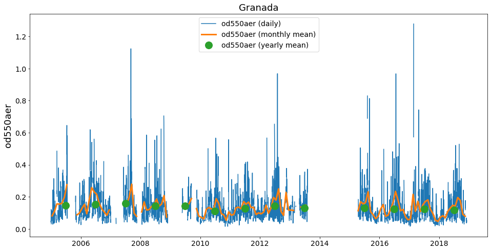
The resampling of the timeseries in the plotting method is done automatically (if input ts_type is provided).
Currently, this does not apply additional constraints such as a minimum number of available observations when downsampling (like we showed above). From the yearly data (green dots) you can see clearly that this can be an issue, especially for the first and the last year.
In order to account for it, you may to the following:
[39]:
# convert to monthly with at least 5 days per month
od550aer_monthly = granada_opt1.resample_timeseries('od550aer', 'monthly', 'mean', min_num_obs=5)

# assign to our StationData
granada_opt1['od550aer_monthly'] = od550aer_monthly

# convert to yearly with at least 6 months per year
od550aer_yearly_constrained = granada_opt1.resample_timeseries('od550aer_monthly', 'yearly', 'mean', min_num_obs=6)
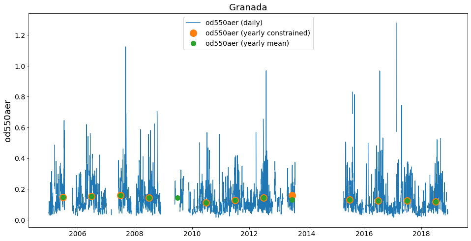
Compare the result with the yearly product plotted above:
[40]:
ax = granada_opt1.plot_timeseries('od550aer')
ax.plot(od550aer_yearly_constrained, ls='none', marker='o', ms=14, label='od550aer (yearly constrained)')
ax = granada_opt1.plot_timeseries('od550aer', freq='yearly', ls='none', marker='o', ms=10, ax=ax)
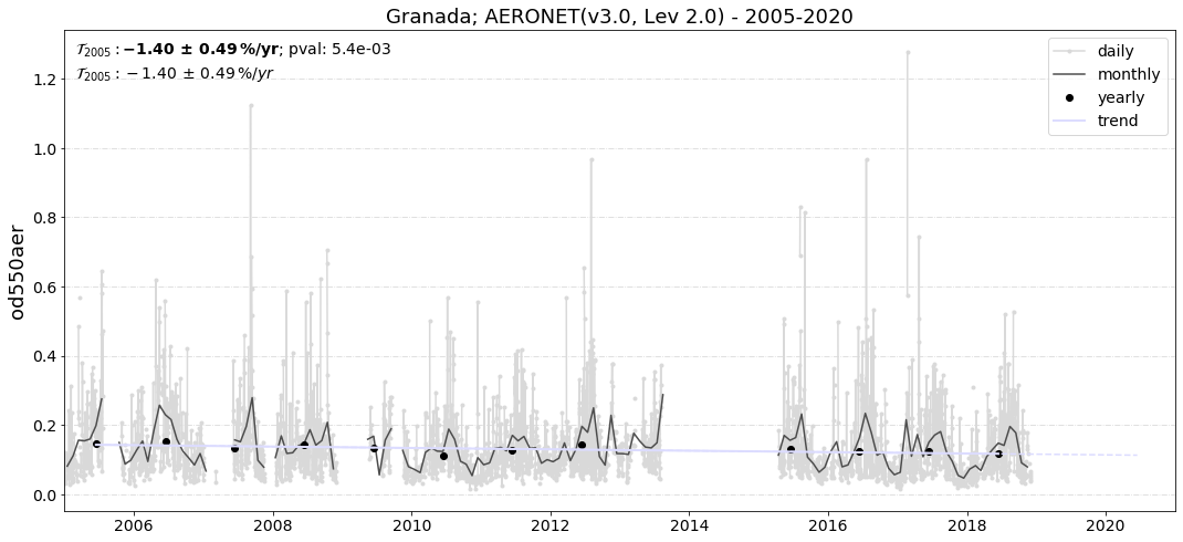
Computing trends from station data
[41]:
granada_opt1.compute_trend(var_name='od550aer', start_year=2005, stop_year=2020)
[41]:
{'pval': 0.005380307706696595,
 'm': -0.0019984909545023464,
 'm_err': 0.0006859706833670536,
 'n': 12,
 'y_mean': 0.13274217888172632,
 'y_min': 0.11068644396371304,
 'y_max': 0.15450395909117362,
 'coverage': None,
 'slp': -1.3972849007872112,
 'slp_err': 0.48509627152652673,
 'reg0': 0.14302673373028105,
 't0': None,
 'slp_2005': -1.3972849007872112,
 'slp_2005_err': 0.48509627152652673,
 'reg0_2005': 0.14302673373028105,
 'yoffs': 0.21297391713786318,
 'period': '2005-2020'}
[42]:
granada_opt1.trends['od550aer'].plot()
[42]:
<matplotlib.axes._subplots.AxesSubplot at 0x7f3a6ccd50b8>